Information Theory in IoT (Part 2)
This is the second part in the Information Theory in IoT series and will discuss converting natural data into independent and identically distributed (IID) values as well as Huffman encoding. The photograph is of of David A. Huffman, developer of Huffman Encoding. Before we get into Huffman encoding though we need to discuss making the data IID.
In this article we’ll address the compression of a single metric, calories per minute. At Nautilus this metric is colloquially called “Burn Rate”. I chose burn rate because of the importance of that particular metric has in our flagship mobile app, JRNY.
Two of the standard methods for achieving IID in a dataset are the Discrete Fourier Transform and the Discrete Cosine Transform. The first is usually applied to a particular metric over time, while the second is applied to a two dimensional array of data. The best example of the latter are RGB values for each pixel in an image when doing JPEG compression. While these methods are industry standards, they are by no means the only means for creating IID data sets. In this example we’ll using an integral transformation of the burn rate. The reason for this is two-fold. First, it will make explanation of the entire process fairly understandable, even to a mathematics laymen such as myself. The second is that even with such a simplistic IID process the compression benefits will be obvious.
The array below is a simplified sample of burn rate data, with each sample taken once per second.
[10,16,14,15,13,13,12,11,13,12,13,14,14,14,13,16,15,14,15,15,15,16,16,16,17,17,18,17,19,21]
The 30 values above, stored as 16 bit integers, normally occupy 480 bits of space. To make the data more IID, we can store the initial value as a 16 bit integer and then take the integral of the remaining values, giving us the discrete rates of change. This gives us the data below:
[10,6,-2,1,-2,|0,-1,-1,2,-1,1,1|,0,0,-1,3,-1,-1|,1,0,0,1,0,0,1|,0,1,-1,2,2]
The Huffman encoding algorithm involves taking values from a set of data and assigning each value a leaf in a binary tree. To maximize the data savings, the most common values are placed closer to the root node of a tree. The simplest rules for generating a Huffman tree use a priority queue for assigning leaf locations, with lowest probability nodes given highest priority. In a queue, FIFO (first in, first out) priority is applied. But in a priority queue this rule is only used for breaking ties in priority. In our example the highest priority is a tie between the values 3 & 6, so those values would be added to the front of the queue. Once the queue is populated the following rules are applied.
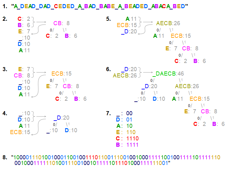
- Create a leaf node for each symbol and add it to the priority queue.
- While there is more than one node in the queue:
- Add the two nodes of highest priority from the queue to the tree as branches.
- Create a new internal node with these two nodes as children and with probability equal to the sum of the two nodes' probabilities.
- Add the new node to the queue.
- Repeat until there are no nodes remaining in the priority queue
- The remaining node is the root node and the tree is complete.
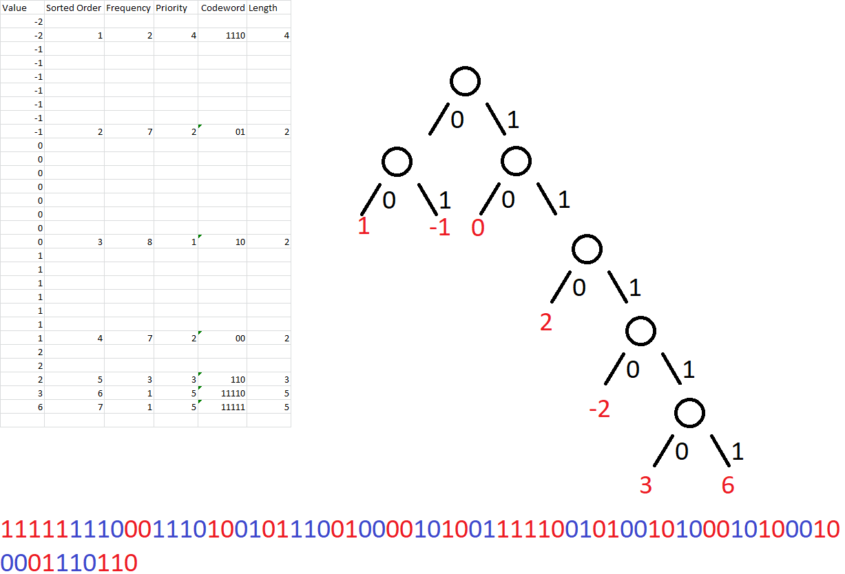
This algorithm is visually depicted above, while the application of those rules is depicted to the left. Each digit is shown as an alternating red or blue set of bits to assist with visually parsing the data. The total number of bits is 71. Adding the 16 bits for the unsigned integer encoding of the initial burn rate value, the application of IID and Huffman encoding has reduced the number of bits from our initial 480 bits to only 87 compressed bits, for a reduction in size of 82%. Another way to look at it is that with 30 integer values represented by 71 bits, each value requires only 2.36 binary digits to be represented, as opposed to the 16 bits of the original, uncompressed encoding.
Now there is one huge asterisk for this compression ratio. That is that this Huffman encoding example is for a very specific set of data. In order to be able to encode and decode a more generalized set of data we would need to capture all the possible changes in burn rate for all of the workouts recorded. Given the wide spectrum of possible values we would want to cap the amount of change between data points in order to limit the total number of values that we would need to generate codewords for. Doing so of course limits the fidelity of the data. But this limitation is relatively minor compared to the fact that we can now store up to five times as many workouts (keeping the length of the workouts constant) than we could previously.
Image credit to https://www.cise.ufl.edu/~manuel/huffman/press.release.html
comments powered by Disqus